
This article was first published on bicorner.com
The following is an excerpt from Predictive Analytics using R, Copyright 2015 by Jeffrey Strickland
In machine learning, Naïve Bayes classifiers are a family of simple probabilistic classifiers based on applying Bayes’ theorem with strong (naïve) independence assumptions between the features.
Naïve Bayes is a popular (baseline) method for text categorization, the problem of judging documents as belonging to one category or the other (such as spam or legitimate, sports or politics, etc.) with word frequencies as the features. With appropriate preprocessing, it is competitive in this domain with more advanced methods including support vector machines (Rennie, Shih, Teevan, & Karger, 2003).
Training Naïve Bayes can be done by evaluating an approximation algorithm in closed form in linear time, rather than by expensive iterative approximation.
Introduction
In simple terms, a Naïve Bayes classifier assumes that the value of a particular feature is unrelated to the presence or absence of any other feature, given the class variable. For example, a fruit may be considered to be an apple if it is red, round, and about 3” in diameter. A Naïve Bayes classifier considers each of these features to contribute independently to the probability that this fruit is an apple, regardless of the presence or absence of the other features.
For some types of probability models, Naïve Bayes classifiers can be trained very efficiently in a supervised learning setting. In many practical applications, parameter estimation for Naïve Bayes models uses the method of maximum likelihood; in other words, one can work with the Naïve Bayes model without accepting Bayesian probability or using any Bayesian methods.
Despite their naïve design and apparently oversimplified assumptions, Naïve Bayes classifiers have worked quite well in many complex real-world situations. In 2004, an analysis of the Bayesian classification problem showed that there are sound theoretical reasons for the apparently implausible efficacy of Naïve Bayes classifiers (Zhang, 2004). Still, a comprehensive comparison with other classification algorithms in 2006 showed that Bayes classification is outperformed by other approaches, such as boosted trees or random forests (Caruana & Niculescu-Mizil, 2006).
An advantage of Naïve Bayes is that it only requires a small amount of training data to estimate the parameters (means and variances of the variables) necessary for classification. Because independent variables are assumed, only the variances of the variables for each class need to be determined and not the entire covariance matrix.
Discussion
Despite the fact that the far-reaching independence assumptions are often inaccurate, the Naïve Bayes classifier has several properties that make it surprisingly useful in practice. In particular, the decoupling of the class conditional feature distributions means that each distribution can be independently estimated as a one-dimensional distribution. This helps alleviate problems stemming from the curse of dimensionality, such as the need for data sets that scale exponentially with the number of features. While Naïve Bayes often fails to produce a good estimate for the correct class probabilities, this may not be a requirement for many applications. For example, the Naïve Bayes classifier will make the correct MAP decision rule classification so long as the correct class is more probable than any other class. This is true regardless of whether the probability estimate is slightly, or even grossly inaccurate. In this manner, the overall classifier can be robust enough to ignore serious deficiencies in its underlying naïve probability model. Other reasons for the observed success of the Naïve Bayes classifier are discussed in the literature cited below.
Example Using R
The Iris dataset is pre-installed in R, since it is in the standard datasets package. To access its documentation, click on ‘Packages’ at the top-level of the R documentation, then on ‘datasets’ and then on ‘iris’. As explained, there are 150 data points and 5 variables. Each data point concerns a particular iris flower and gives 4 measurements of the flower: Sepal.Length, Sepal.Width, Petal.Length and Petal.Width together with the flower’s Species. The goal is to build a classifier that predicts species from the 4 measurements, so species is the class variable.
To get the iris dataset into your R session, do:
> data(iris)
at the R prompt. As always, it makes sense to look at the data. The following R command (from the Wikibook) does a nice job of this.
> pairs(iris[1:4],main=“Iris Data
 +   (red=setosa,green=versicolor,blue=virginica)”, pch=21,
 +   bg=c(“red”,”green3”,”blue”)[unclass(iris$Species)])
The ‘pairs’ command creates a scatterplot. Each dot is a data point and its position is determined by the values that data point has for a pair of variables. The class determines the color of the data point. From the plot note that Setosa irises have smaller petals than the other two species.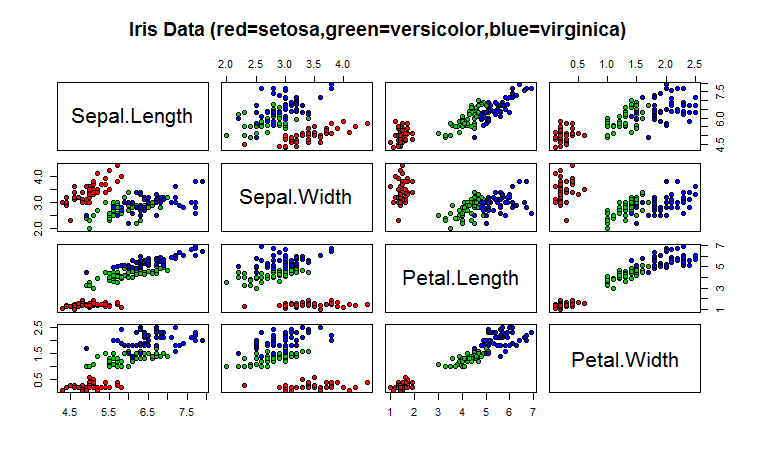
> summary(iris)
provides a summary of the data.Typing:Sepal.Length Sepal.Width Petal.Length Petal.Width Species
Min. :4.300 Min. :2.000 Min. :1.000 Min. :0.100 setosa :50
1st Qu.:5.100 1st Qu.:2.800 1st Qu.:1.600 1st Qu.:0.300 versicolor:50
Median :5.800 Median :3.000 Median :4.350 Median :1.300 virginica :50
Mean :5.843 Mean :3.057 Mean :3.758 Mean :1.199
3rd Qu.:6.400 3rd Qu.:3.300 3rd Qu.:5.100 3rd Qu.:1.800
Max. :7.900 Max. :4.400 Max. :6.900 Max. :2.500
> iris
Prints out the entire dataset to the screen.
Sepal.Length  Sepal.Width   Petal.Length  Petal.Width     Species
 1        5.1          3.5            1.4          0.2      setosa
 2        4.9          3              1.4          0.2      setosa
 3        4.7          3.2            1.3          0.2      setosa
 4        4.6          3.1            1.5          0.2      setosa
 5        5            3.6            1.4          0.2      setosa
 -----------------------------Data omitted-------------------------
 149      6.2          3.4            5.4          2.3      virginica
 150      5.9          3              5.1          1.8      virginica
Constructing a Naïve Bayes classifier
We will use the e1071 R package to build a Naïve Bayes classifier. Firstly you need to download the package (since it is not pre-installed here). Do:
> install.packages(“e1071”)
Choose a mirror in US from the menu that will appear. You will be prompted to create a personal R library (say yes) since you don’t have permission to put e1071 in the standard directory for R packages.
To (1) load e1071 into your workspace (2) build a Naïve Bayes classifier and (3) make some predictions on the training data, do:
> library(e1071)
> classifier<-naivebayes br="" iris="">> table(predict(classifier, iris[,-5]), iris[,5],
 +     dnn=list(‘predicted’,’actual’))
As you should see the classifier does a pretty good job of classifying. Why is this not surprising?
predicted   setosa versicolor virginica
 setosa          50          0         0
 versicolor       0         47         3
 virginica        0          3        47
To see what’s going on ‘behind-the-scenes’, first do:
> classifier$apriori
This gives the class distribution in the data: the prior distribution of the classes. (‘A priori’ is Latin for ‘from before’.)
iris[, 5]
 setosa  versicolor  virginica
 50          50         50
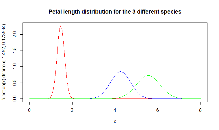
Since the predictor variables here are all continuous, the Naïve Bayes classifier generates three Gaussian (Normal) distributions for each predictor variable: one for each value of the class variable Species. If you type:
> classifier$tables$Petal.Length
You will see the mean (first column) and standard deviation (second column) for the 3 class-dependent Gaussian distributions:
 Petal.Length
 iris[, 5]    [,1]       [,2]
 setosa      1.462  0.1736640
 versicolor  4.260  0.4699110
 virginica   5.552  0.5518947
You can plot these three distributions against each other with the following three R commands:
> plot(function(x) dnorm(x, 1.462, 0.1736640), 0, 8,
 +   col=“red”, main=“Petal length distribution for the 3
 +   different species”)
>  curve(dnorm(x, 4.260, 0.4699110), add=TRUE, col=“blue”)
>  curve(dnorm(x, 5.552, 0.5518947), add=TRUE, col=“green”)
Note that setosa irises (the red curve) tend to have smaller petals (mean value = 1.462) and there is less variation in petal length (standard deviation is only 0.1736640).
Understanding Naïve Bayes
In the previous example you were given a recipe which allowed you to construct a Naïve Bayes classifier. This was for a case where we had continuous predictor variables. In this question you have to work out what the parameters of a Naïve Bayes model should be for some discrete data.
The dataset in question is called HairEyeColor and has three variables: Sex, Eye and Hair, giving values for these 3 variables for each of 592 students from the University of Delaware. First have a look at the numbers:
You can also plot it as a ‘mosaic’ plot which uses rectangles to represent the numbers in the data:> HairEyeColor
, , Sex = Male
Eye
 Hair   Brown Blue Hazel Green
 Black     32   11    10     3
 Brown     53   50    25    15
 Red       10   10     7     7
 Blond      3   30     5     8
, , Sex = Female
Eye
 Hair   Brown Blue Hazel Green
 Black     36    9     5     2
 Brown     66   34    29    14
 Red       16    7     7     7
 Blond      4   64     5     8
> mosaicplot(HairEyeColor)
Mosaic plot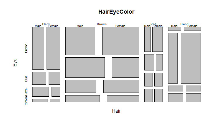
Your job here is to compute the parameters for a Naïve Bayes classifier which attempts to predict Sex from the other two variables. The parameters should be estimated using maximum likelihood. To save you the tedium of manual counting, here’s how to use margin.table to get the counts you need:
> margin.table(HairEyeColor,3)
  Sex
 Male Female
 279     313
> margin.table(HairEyeColor,c(1,3))Sex
Hair Male Female
Black 56 52
Brown 143 143
Red 34 37
Blond 46 81
Note that Sex is variable 3, and Hair is variable 1. Once you think you have the correct parameters speak to me or one of the demonstrators to see if you have it right. (Or if you can manage it, construct the Naïve Bayes model using the naiveBayes function and yank out the parameters from the model. Read the documentation to do this.)
We can also perform Naïve Bayes with the Classification and Visualization (klaR) package which was not covered in this article.
Authored by: Jeffrey Strickland, Ph.D.
Jeffrey Strickland, Ph.D., is the Author of Predictive Analytics Using R and a Senior Analytics Scientist with Clarity Solution Group. He has performed predictive modeling, simulation and analysis for the Department of Defense, NASA, the Missile Defense Agency, and the Financial and Insurance Industries for over 20 years. Jeff is a Certified Modeling and Simulation professional (CMSP) and an Associate Systems Engineering Professional (ASEP). He has published nearly 200 blogs on LinkedIn, is also a frequently invited guest speaker and the author of 20 books including:
- Operations Research using Open-Source Tools
- Discrete Event simulation using ExtendSim
- Crime Analysis and Mapping
- Missile Flight Simulation
- Mathematical Modeling of Warfare and Combat Phenomenon
- Predictive Modeling and Analytics
- Using Math to Defeat the Enemy
- Verification and Validation for Modeling and Simulation
- Simulation Conceptual Modeling
- System Engineering Process and Practices
No comments:
Post a Comment